Fits continuous trajectory interpolating curves from GTFS schedule data.
Source:R/trajectory_constructors.R
get_gtfs_trajectory_fun.RdThis function fits a continuous vehicle trajectory function to scheduled GTFS
stop_times, returning a trajectory object. Interpolation can be done
linearly (interp_method = "linear"), or via any method supported by
stats::splinefun().
Usage
get_gtfs_trajectory_fun(
  gtfs,
  shape_geometry = NULL,
  project_crs = 4326,
  date_min = NULL,
  date_max = NULL,
  use_calendar_table = "calendar",
  agency_timezone = NULL,
  use_stop_time = "departure",
  add_stop_dwell = 0,
  add_distance_error = 0,
  interp_method = "linear",
  find_inverse_function = TRUE,
  return_group_function = TRUE,
  inv_tol = 0.01
)
Arguments
- gtfs
A tidygtfs object.
- shape_geometry
Optional. The SF object to project onto. Must include the field
shape_id. Seeget_shape_geometry(). Default isNULL, where all shapes ingtfswill be used.- project_crs
Optional. A numeric EPSG identifer indicating the coordinate system to use for spatial calculations. Consider setting to a Euclidian projection, such as the appropriate UTM zone. Default is 4326 (WGS 84 ellipsoid).
- date_min
Optional. The starting (earliest possible) Date object for the returned dataframe. Default is
NULL, where the earliest date in the GTFS will be used.- date_max
Optional. The ending (latest possible) Date object for the returned dataframe. Default is
NULL, where the latest date in the GTFS will be used.- use_calendar_table
Optional. Should the GTFS's
calendar.txtorcalendar_dates.txtbe used for the feasible date range? Must be"calendar"or"calendar_dates". Default is"calendar".- agency_timezone
Optional. A timezone string (see
OlsonNames()) indicating he appropriate timezone for the stop times. Default isNULL, where the timezone inagency.txtwill be used.- use_stop_time
Optional. A string, which stop time column should be used for the timepoint? Must be one of
"arrival"(usearrival_time),"departure"(usedeparture_time), or"both", (timepoints will be created at both the stop arrival and departure). Default is"departure".- add_stop_dwell
Optional. A numeric. If
use_stop_time = "both", but scheduled arrival and departure times are equal (i.e., no dwell), how many seconds of dwell should be added? This will adjust forward thedeparture_time. Default is 0.- add_distance_error
Optional. If non-zero, each "flat" observation will be adjusted by this amount forwards, in units of input
distance. Default is 0.- interp_method
Optional. The type of interpolation function to be fit. Either
"linear", or a spline method fromstats::splinefun(). Default is"linear".- find_inverse_function
Optional. A boolean, should the numeric inverse function (time ~ distance) be calculated? Default is
TRUE.- return_group_function
Optional. A boolean, should the returned trajectory object be grouped into a single function? If FALSE, will return a list (indexed by
trip_id_performed) of single trajectory objects. Default isTRUE.- inv_tol
Optional. A numeric in the units of input
distance, the tolerance used when calculating the numeric inverse function. Default is 0.01.
Value
If return_group_function = TRUE, a grouped trajectory object. If
FALSE, a list of single trajectory objects, index by their
trip_id_performed.
Details
Stops, Dwells, and Monotonicity
To fit an interpolating trajectory function, each observation must include
distance and timestamp pairs throughout each trip. While stop_times does
include a shape_dist_traveled field, this is optional and often left
empty by agencies. Additionally, small distortions in spatial projections
mean that projected GPS points may not align perfectly with the agency's
calculated shape_dist_traveled. As such, this function uses
get_stop_distances() to get the distance of each stop along each shape for
each trip. Alternatively, all stops and trips can be referenced to the
same spatial feature using shape_geometry. Consider setting project_crs
to the same spatial projection used to linearize AVL GPS points.
The trajectory functions are fit using the times a trip is scheduled to
serve each stop. There is some ambiguity here: should a stop's timestamp
be when the vehicle arrives, or departs? This can be controlled using
use_stop_time, set to "departure" for departure_time, "arrival" for
arrival_time, or "both" to include both departure_time and
arrival_time as distinct observations (i.e., distance & timestamp pairs).
Often times, however, a GTFS schedule will not have different arrival_time
and departure_time values, especially if the timetable was not developed
considering stop-level dwell times. In this scenario, it may be best to use
only one of departure_time or arrival_time. If a dwell is desired, use
add_stop_dwell to simulate a dwell time at each stop. This will increase
the departure_time by the number of seconds specified.
Adding dwells opens a new consideration, however: the trajectory will no
longer be strictly monotonic, as the vehicle will hold at a constant distance
for some period of time. This is only a concern if
find_inverse_function = TRUE, which requires strictly monotonic input data.
If both dwell times and an inverse function are desired, consider setting
add_distance_error > 0 to restore strict monotonicity. See
make_monotonic() for more details.
Interpolating Methods
The goal of this function is to fit a continuous function representing a GTFS trip's scheduled distance traveled as a function of time. This function supports to types of interpolating curves:
Linear interpolation, for
interp_method = "linear". This will fit a simple linear function, ignorant of recordedspeedvalues.Spline interpolation, for
interp_methodset to any method supported bystats::splinefun()(i.e.,"fmm","natural","periodic","monoH.FC", or"hyman".)
By default, interp_method = linear, and linear interpolation is the
recommended method for schedule trajectories. This is because timetable
development typically assumes a constant running speed over a corridor, so
linearly connecting stop times will best reflect a trip's scheduled
trajectory.
Inverse Functions
Often times, we are concerned not with the position of a vehicle at a
particular time, but when a vehicle crosses a specific point in space. This
can be accomplished by computing an inverse trajectory function. If
find_inverse_function = TRUE (the default), a numeric inverse to the fit
trajectory function will be found, with a tolerance controlled by inv_tol.
Because the inverse function is numerical, it can be found for any type of
interpolating curve (linear or spline). However, the input data must be
strictly monotonic for the trajectory curve to be invertible. If
find_inverse_function = TRUE, this will be verified before proceeding (see
validate_monotonicity()).
The Trajectory Object
A trajectory function does not exist by itself; rather, it requires the
context about the trip it describes, as well as its inverse function. As
such, get_trajectory_fun() returns an AVL trajectory object. If
return_group_function = TRUE (the default), the function will return a
single object containing:
A vector of
trip_id_performeds, from thetrip_ids found intrips.A list of fit trajectory functions, indexed by their
trip_id_performed.A list of fit inverse trajectory functions, indexed by their
trip_id_performed.Information about how the trajectory and inverse trajectory functions were fit, including
interp_method,use_speeds, andinv_tol.A vector each for the minimum distances, maximum distances, minimum times, and maximum times of each trip. These inform the domain and range of the trajectory function and its inverse, preventing extrapolation beyond the time or distance range actually served by a trip.
Alternatively, if return_group_function = FALSE, a separate trajectory
object will be fit for each trip. get_trajectory_fun() will return a list
of trajectory objects indexed by their trip_id_performed.
More information about the trajectory object classes and how to use them is available at (xyz).
Examples
# Set my parameters
my_crs <- 32618
my_start_date <- as.Date("2026-02-16")
my_end_date <- as.Date("2026-02-16")
# Get input data
c53_gtfs <- new_transittraj_data("filter_by_route")
c53_shape <- new_transittraj_data("get_shape_geometry")
# Run function: build trajectory
c53_scheduled_traj <- get_gtfs_trajectory_fun(gtfs = c53_gtfs,
project_crs = my_crs,
date_min = my_start_date,
date_max = my_end_date)
# Show trajectory: summary & plot
summary(c53_scheduled_traj)
#> ------
#> AVL Group Trajectory Object
#> ------
#> Number of trips: 108
#> Total distance range: 2.073578 to 15463.51
#> Total time range: 1771221600 to 1771310100
#> ------
#> Trajectory function present: TRUE
#> --> Trajectory interpolation method: linear
#> --> Maximum derivative: 0
#> --> Fit with speeds: FALSE
#> Inverse function present: TRUE
#> --> Inverse function tolerance: 0.01
#> ------
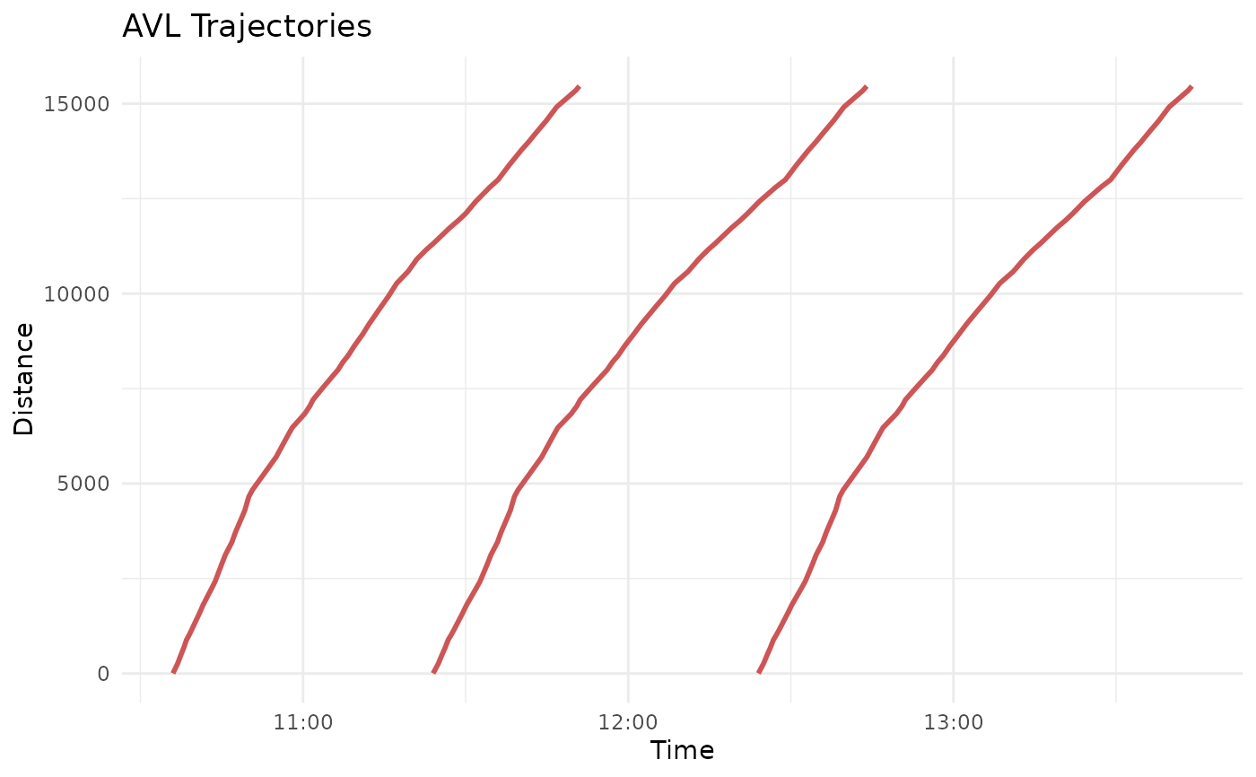
plot_trajectory(trajectory = c53_scheduled_traj,
plot_trips = unclass(c53_scheduled_traj)[8:10],
traj_color = "indianred3")